
Convolutional neural networks have achieved the best results in machine vision and many other problems. Its success has prompted us to think about a problem. Why is convolutional neural networks so effective? In this article, SIGAI will analyze the mysteries behind the convolutional neural network for everyone.
Origin of thought
Among various deep neural network structures, convolutional neural networks are the most widely used ones, which were proposed by LeCun in 1989 [1]. Convolutional neural networks were successfully applied to handwritten character image recognition in the early days. In 2012, the deeper AlexNet network[4] succeeded. Since then, the convolutional neural network has been booming. It has been widely used in various fields and has achieved the best performance on many issues.
The convolutional neural network automatically learns the features of the image at various levels through convolution and pooling operations, which is consistent with our understanding of the image. When people recognize images, they are layered and abstract. The first thing to understand is color and brightness, then the local details such as edges, corners, and lines, followed by more complex information and structures such as textures and geometric shapes. The concept of the entire object.
Visual Neuroscience's research on the visual mechanism verifies this conclusion. The visual cortex of the animal's brain has a layered structure. The eye sees the scene on the retina. The retina converts the optical signal into an electrical signal and passes it to the visual cortex of the brain. The visual cortex is the part of the brain that processes visual signals. In 1959, David and Wiesel conducted an experiment [5]. They inserted electrodes in the primary visual cortex of the cat's brain, displayed light strips of various shapes, spatial positions, and angles in front of the cat's eyes, and then measured the release of cat brain neurons. The electrical signal. Experiments show that when the light band is at a certain position and angle, the electrical signal is the strongest; different neurons have different preferences for various spatial positions and orientations. This achievement later gave them the Nobel Prize.
It has been demonstrated that the visual cortex has a hierarchical structure. The signal from the retina first reaches the primary visual cortex, the V1 cortex. The V1 cortical simple neuron is sensitive to some details, specific direction of the image signal. After the V1 cortex was processed, the signal was transmitted to the V2 cortex. The V2 cortex represents the edge and contour information as a simple shape and is then processed by neurons in the V4 cortex, which is sensitive to color information. Complex objects are finally represented in the inferior temporal cortex.

Visual cortical structure
A convolutional neural network can be seen as a simple imitation of the above mechanism. It is composed of multiple convolution layers. Each convolution layer contains multiple convolution kernels. The convolution kernels scan the entire image from left to right and from top to bottom to obtain a feature map. Output Data. The convolutional layer in front of the network captures image local and detail information and has a small receptive field, ie, each pixel of the output image uses only a small range of the input image. The convolutional layer behind it feels more and more layered and used to capture more complex and more abstract images. After multiple convolutional operations, the abstract representation of the image at different scales is finally obtained.
Convolution operation
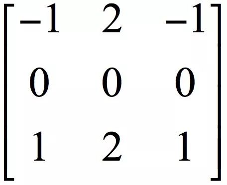
Convolution of one-dimensional signals is a classical method in digital signal processing. In image processing, convolution is also a common operation. It is used for image denoising, enhancement, edge detection, etc. It can also extract image features. The convolution operation uses a matrix called a convolution kernel to slide over the image from top to bottom and from left to right. The elements of the convolution kernel matrix are multiplied with the elements of the convolution kernel in the corresponding positions covered by the image. And, get the output pixel value. Take the Sobel edge detection operator as an example. Its convolution kernel matrix is:
Suppose the matrix of the input image is a 3x3 sub-image centered on (x,y):
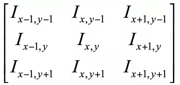
The convolution result at this point is calculated as follows:

That is, the sub-image centered on (x,y) is multiplied by the corresponding element of the convolution kernel and then added. By applying nuclear convolution to all positions of the input image, we can get the edge map of the image. The edge map has a larger value at the edge position and the value at the non-edge is close to zero. The following figure shows the result of the convolution of the Sobel operator on the image. The left image is the input image, and the right image is the convolution result:
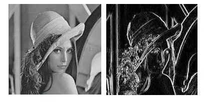
Sobel operator convolution results
As you can see from the above figure, the edge information of the image is highlighted by convolution. In addition to Sobel operators, Roberts, Prewitt operators, etc. are commonly used. They have the same convolution method but different convolution kernel matrices. If we use other different kernels, we can also extract more general image features. In image processing, the values ​​of these convolution kernel matrices are artificially designed. By some method, we can automatically generate these convolution kernels by means of machine learning to describe various types of features. Convolutional neural networks are used to obtain various useful convolution kernels through this automatic learning method. .
Convolution layer
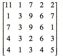
The convolutional layer is the core of the convolutional neural network. The following is a practical example to understand the convolution operation. If the convolved image is:
The convolution kernel is:
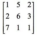
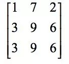
First, the sub-image at the first position of the image, ie, the top-left sub-image and the convolution kernel corresponding elements are multiplied and then added, where the sub-image is:
The result of the convolution is:

Next, slide a column to the right on the image to be convolved, and place the sub-image at the second position:
Convolved with the convolution kernel, the result is 154. Next, slide it to the right again to convolve the sub-image at the third position with the convolution kernel. The result is 166. After processing the first row, swipe down one line and repeat the process above. And so on, the final image of the convolution result is:
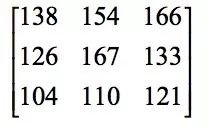
After convolution, the image size becomes smaller. We can also perform padding on the image first, for example by adding zeros to the periphery, and then convolving the image with the enlarged size to ensure that the convolution result image is the same size as the original image. In addition, in the process of sliding from left to right from top to bottom, the horizontal and vertical sliding steps are all 1, we can also use other steps.
The convolution operation is obviously a linear operation, and the neural network must be fitted with a nonlinear function. Therefore, similar to a full-connection network, we need to add an activation function. Commonly used are sigmoid functions, tanh functions, and ReLU functions. For the explanation of the activation function, why activate the function and what kind of function can be used as the activation function, SIGAI will be described in the follow-up article, please pay attention to our public number.
We talked about the convolution of single-channel images. The input is a two-dimensional array. In practice, we often encounter multi-channel images. For example, RGB color images have three channels. In addition, since each layer can have multiple convolution kernels, the resulting output is also a multi-channel feature image. This corresponds to the convolution. The core is also multi-channel. The specific method is to convolve each channel of the input image with each channel of the convolution kernel and then accumulate the pixel values ​​at the corresponding positions according to each channel.
Since multiple convolution kernels are allowed in each layer, multiple feature images are output after the convolution operation. Therefore, the number of convolution kernel channels in the L convolution layer must be the same as the number of channels in the input feature image, that is, equal to the L-th The number of convolution kernels in a convolutional layer.
The following figure is a simple example:
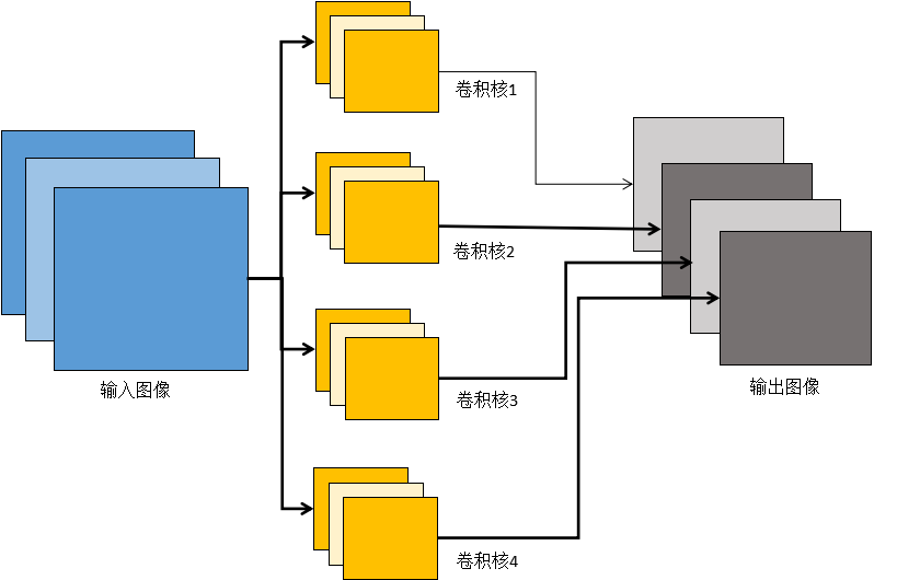
Multi-channel convolution
In the figure above, the input image of the convolutional layer is 3-channel (column 1 in the figure). Correspondingly, the convolution kernel is also 3-channel. In the convolution operation, the convolutions of the respective channels are respectively convolved with the convolution of each channel, and then the respective channel values ​​at the same position are accumulated to obtain a single channel image. In the figure above, there are 4 convolution kernels. Each convolution kernel produces a single-channel output image. Four convolution kernels produce a total of 4 channel output images.
Pooling layer
Through the convolution operation, we have completed the dimension reduction and feature extraction of the input image, but the dimension of the feature image is still very high. The high dimension is not only time-consuming but also easily leads to overfitting. To this end, a downsampling technique has been introduced, also known as pooling or pooling operations.
Pooling is done by replacing one area of ​​the image with a value, such as a maximum or average value. If you use the maximum value, it is called max pooling; if you use the average, it is called mean pooling. In addition to reducing the image size, another benefit of downsampling is translation and rotation invariance, because the output value is calculated from one area of ​​the image and is not sensitive to translation and rotation.
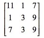
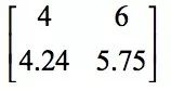
Below is a practical example to understand the downsampling operation. The input image is:
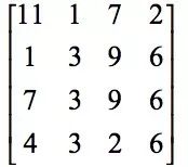
Non-overlapped 2x2max pooling here, the resulting image is:

The first element 11 in the resulting image is the 2x2 sub-image in the top left corner of the original image:

The maximum value of the element is 11. The second element 9 is the second 2x2 sub-image:

The maximum value of the element is 9, and so on. If you are using a mean downsampling, the result is:
The concrete implementation of the pooling layer is to block the obtained feature image after the convolution operation, and the image is divided into disjoint blocks, and the maximum or average value in these blocks is calculated to obtain the pooled image.
Both the pooling of the mean and the pooling of max can accomplish the downsampling operation. The former is a linear function and the latter is a non-linear function. In general, max pooling has a better effect.
Network structure
A typical convolutional neural network consists of a convolutional layer, a pooled layer, and a fully connected layer. Here is a description of the LeNet5 network. The following figure shows the structure of this network:
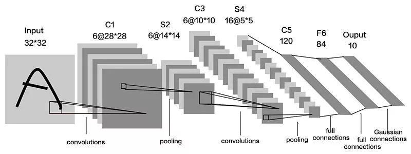
The input gray image of the network consists of 3 convolution layers, 2 pool layers, and 1 fully connected layer. There is a pooling layer behind the first two convolutional layers. The output layer has 10 neurons, representing the 10 numbers 0-9.
application
Machine vision is the first breakthrough in deep learning technology and is the most widely used field. After AlexNet appeared, the convolutional neural network was quickly used for various tasks in machine vision, including general target detection, pedestrian detection, face detection, face recognition, image semantic segmentation, edge detection, target tracking, and video classification. All kinds of problems have been successful.
Most problems in the field of natural language processing are time series problems, which are problems that a recurrent neural network is good at. But for some problems, the use of convolutional networks can also be modeled and the results are very good, typically text categorization and machine translation.
In addition, convolutional neural networks have applications in speech recognition, computer graphics, and other directions.
Convolutional visualization
The original intention of the convolutional network design is to gradually extract the features of the image at different levels of abstraction through the convolutional layer and the pooled layer. We will have such questions: Is the actual result really like this?
Look at the results after the image convolution. Here is an image of a truck:
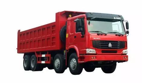
Truck image
After processing with the AlexNet network, the output of the first convolutional layer (we've ordered the results of each convolution kernel in turn) is like this:
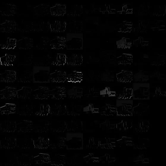
Results of Volume 1
You can see some edge information extracted here. The output of the second convolutional layer looks like this:
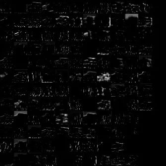
Layer 2 results
It extracts features of a larger area. The result of the following several convolutional layers is this:

Results of Volume 3-5
The results of the convolution layers 3-5 are successively arranged in the figure above. Then we look at the full connection layer. The following figure shows the output of 3 fully connected layers from top to bottom:
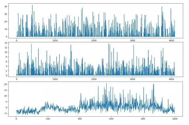
Fully connected layer results
Let us look at the visualization of the convolution kernel. The first convolutional convolution kernel image is shown below:

Convolution kernel of convolution 1
It can be seen that these convolution kernels are indeed in the extraction of edges, directions, and other information. Look at the second convolutional convolution kernel:
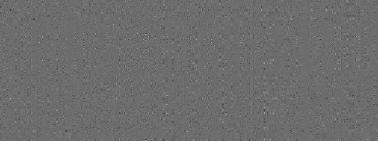
Convolution kernel 2 convolution kernel
It looks very messy and doesn't respond to too much information. Is there a better way? The answer is yes, and there are a number of articles that address the issue of visualization of convolutional layers. Here, we introduce a typical method to visualize the effect of a convolution kernel by deconvolution.
Document [6] designed a scheme for visualizing convolutional layers using deconvolution. The specific approach is to multiply the feature images learned by the convolutional network by the transpose matrix of the convolution kernels of these feature images and project the picture features from the feature image space to the pixel space to find out which pixels activate specific features. The image is analyzed to understand the purpose of the convolutional network. This operation is called deconvolution, also called transposition convolution.
For a convolutional layer, a convolution kernel of the convolution kernel in the forward propagation is used to convolute the feature image during deconvolution operation, and the feature image is restored to the original pixel image space to obtain a reconstructed image. The visual image of the convolution kernel obtained by the deconvolution operation is shown below:
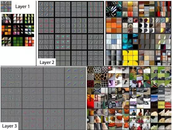
Visualize by deconvolution
The above figure shows that the features extracted by the previous layer are relatively simple and are some colors and edge features. The more complex the features extracted from the convolutional layer are, the more complex geometric shapes are. This is in line with our original intention of designing a convolutional neural network, that is, to perform layer-by-layer feature extraction and abstraction of images through multi-level convolution.
Another method to analyze the mechanism of the convolutional network is to reconstruct the original input image directly based on the convolution result image. If the original input image can be reconstructed based on the convolution result, the convolution network largely retains the image. information. In [7], a method was designed to observe the convolutional network's expressive ability by inversely expressing the features extracted from the convolutional network. Here, the reverse representation means that the original input image is approximately reconstructed by a convolutional network-encoded vector. The specific approach is to give a convolutional network coded vector, look for an image, this image through the convolutional network encoding the vector and the given vector best match, this is achieved by solving an optimization problem. The following figure is an image reconstructed from the convolution output result:
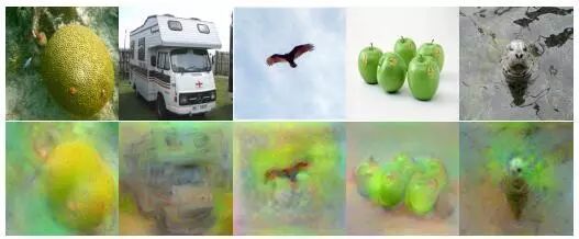
Convolution image reconstruction
Among them, the top row is the original image, and the bottom row is the reconstructed image. From this result, it can be seen that the convolutional neural network does extract the useful information of the image.
theoretical analysis
The theoretical explanation and analysis of convolutional neural networks comes from two aspects. The first aspect is the analysis from the mathematical point of view, the mathematical analysis of the network's representation ability and mapping characteristics; the second aspect is the study of the relationship between the convolutional network and the animal vision system. Analyzing the relationship between the two is helpful for understanding and designing. A better approach, at the same time, also promotes the advancement of neuroscience.
Mathematical characteristics
The neural network represents the connectionist idea in artificial intelligence. It is a bionic method and is considered as a simulation of the nervous system of animal brains. When it is implemented, it is different from the structure of the brain. From a mathematical point of view, multilayer neural networks are essentially a complex function.
Since neural networks are essentially complex complex functions, this leads us to consider one question: How strong is the function of modeling this function? What kind of objective function can it simulate? It has been proved that as long as the activation function is properly selected and the number of neurons is sufficient, the use of a 3-layer neural network containing a hidden layer can achieve approximation of any continuous mapping function from the input vector to the output vector [8][ 9][10], this conclusion is called the universal approximation theorem.
The literature [10] proves the situation when using the sigmoid activation function. The literature [8] pointed out that the universal approximation property does not depend on the specific activation function of the neural network, but is guaranteed by the structure of the neural network.
The expression of the universal approximation theorem is: If 


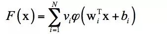
For any 
The intuitive explanation of the universal approximation theorem is that it is possible to construct a function such as the above, which approximates any continuous function defined in the unit cubic space to any given precision. This conclusion is similar to the polynomial approximation, which uses a polynomial function to approximate any continuous function to any precision. The significance of this theorem is that it theoretically guarantees the fitting ability of the neural network.
However, this is only a theoretical result. How many layers do the neural networks require and how many neurons need to be on each layer? These problems can only be determined by experiment and experience to ensure the effect. Another problem is training samples. To fit a complex function requires a large number of training samples and faces the problem of overfitting. The details of the implementation of these projects are also crucial. The convolution network has been around since 1989. Why did it not succeed until 2012? There are several points in the answer:
1. Limit the number of training samples. The early training samples were very few and there was no large-scale collection. It was not enough to train a complicated convolutional network.
2. Limits on computing power. The computer capabilities of the 1990s were too weak. Without high-performance computing technologies such as GPUs, training a complex neural network was unrealistic.
3. The algorithm itself. For a long time, the neural network has the problem of gradient disappearing. Because each layer must be multiplied by the derivative value of the activation function in the backward propagation, if the absolute value of this derivative is less than 1, the gradient will soon approach 0 after many times. The previous layer cannot be updated.
The size of the AlexNet network, especially the number of layers deeper than the previous network, uses ReLU as an activation function, abandoning the sigmoid and tanh functions, to some extent ease the gradient disappearance problem. Coupled with the Dropout mechanism, it also alleviates over-fitting problems. These technical improvements, coupled with large sample sets such as ImageNet, and the computational power of the GPU, ensure its success. Later research shows that increasing the number of layers and parameters of the network can significantly increase the accuracy of the network. For these issues, SIGAI will be detailed in the following feature articles, and interested readers can pay attention to our public number.
A convolutional neural network is essentially a weighted shared fully connected neural network, so the universal approximation theorem is applicable to it. However, the convolutional layer and pooled layer of the convolutional network have their own characteristics. The literature [11] explains the deep convolutional network from the mathematical point of view. Here, the author considers the convolutional network as a set of cascaded linear weighted filters and nonlinear functions to scatter the data. The analysis of the contraction and separation features of this set of functions explains the modeling capabilities of the deep convolutional network. In addition, the migration characteristics of deep neural networks are also explained. Convolutional neural network convolution operation is divided into two steps, the first step is a linear transformation, the second step is to activate the function transformation. The former can be seen as linear projection of data to a lower dimensional space; the latter is a compression nonlinear transformation of data. The author analyzes the separation and compression characteristics of these types of transformations.
Relationship with the visual nervous system
The relationship between the convolutional network and the human visual system has important implications for the interpretation and design of convolutional networks. This is divided into two aspects. The first question is whether deep convolutional neural networks can achieve similar performance to the human brain vision system. This involves comparing the capabilities of the two. The second question is whether there is consistency in the structure between the two, which is to analyze the relationship between the two from the system structure.
From a deeper perspective, this issue is also an issue that artificial intelligence cannot avoid. Many people will have a question: Do we have to understand the working mechanism of the brain to achieve its artificial intelligence? There are two opinions on the answer to this question. The first view is that we must first understand the principle of the brain in order to develop artificial intelligence that is equivalent to his function. The second view is that even if we do not understand the working principle of the brain, we can develop artificial intelligence that is equivalent to its ability. One example is the invention of the aircraft. For a long time, people wanted to create airplanes by mimicking the way a bird flies, that is, flapping its wings. The results all ended in failure. The use of propellers allows us to use another method, but also allows the aircraft to fly up, the jet engine behind us even let us break the speed of sound, far more powerful than the bird. In fact, the brain may not be the only solution for achieving intelligence that is equivalent to it.

They verified that deep neural networks can achieve the same performance as primate visual IT cortex. The human brain's visual nervous system can still achieve high recognition performance in the case of object changes, geometric transformations, and background changes. This is mainly attributable to the inferior temporal cortex of the inferior temporal cortex, the abilities of the IT cortex. Through the deep convolutional neural network training model, high performance is also achieved on the object recognition problem. There are many difficulties in accurately comparing the two.
The authors compared deep neural networks with the IT cortex using expanded nuclear analysis techniques. This technique uses the model's generalization error as a function of complexity. The analysis results show that the performance of the deep neural network in the task of visual target recognition can be expressed in the cerebral cortex.
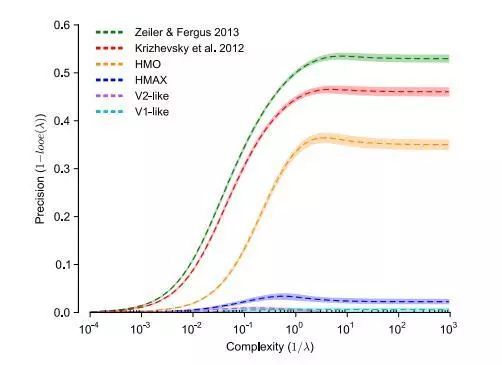
Neural Network and Visual Cortical Ability Comparison
The correspondence between the deep neural network and the optic nerve. They use a goal-driven deep learning model to understand the sensory cortex of the brain. The specific idea is to use goal-driven hierarchical convolutional neural networks (HCNNs) to model the output responses of individual units and groups in the high visual cortex area. This approach establishes a corresponding relationship between deep neural networks and the cerebral cortex, which can help us understand the mechanism of the visual cortex. From another point of view, we have also found the corresponding point of deep neural network in neuroscience. The following figure shows the structure and function of neural networks and visual cortex:
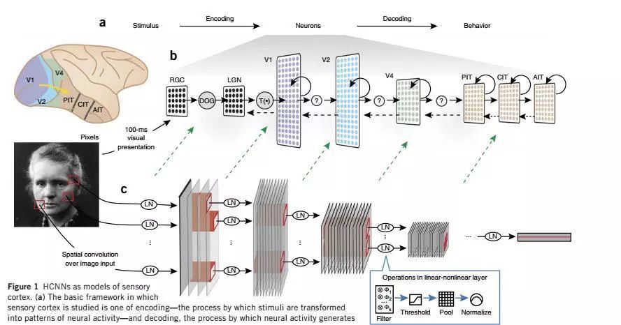
Neural Network and Visual Cortical Structure Comparison
At present, the research on the working mechanism and theory of deep neural networks is not perfect, and the study of brain science is still at a relatively low level. It is believed that in the future through continuous human efforts, the working mechanism of the brain can be understood more clearly and a more powerful neural network can be designed.
Antenk Insulation Displacement termination connectors are designed to quickly and effectively terminate Flat Cable in a wide variety of applications. The IDC termination style has migrated and been implemented into a wide range of connector styles because of its reliability and ease of use. Click on the appropriate sub section below depending on connector or application of choice.
An insulation-displacement contact (IDC), also known as insulation-piercing contact (IPC), is an electrical connector designed to be connected to the conductor(s) of an insulated cable by a connection process. The IDC forces a selectively sharpened blade or blades through the insulation, bypassing the need to strip the cable.

IDC Plug / Socket - Card Edge Slot Connector
Card Edge SLOT Connector is the portion of a printed circuit board (PCB) consisting of traces leading to the edge of the board that are intended to plug into a matching socket.
IDC Connectors
The IDC connector is also known as an insulation-displacement contact, or insulation-piercing contact. It is a connector designed to work with ribbon cables, and uses sharp contacts to clamp onto the wire, piercing the insulation and connecting with the wire in a secure and convenient way.
This simple connection principle is ideal for multi-stranded ribbon cables, as it allows the connector to make an assured connection across the multiple wires without having to strip the wires. This cold welding connection may ensure a gas tight connection between the wire and connector.
The Antenk range of IDC connectors includes plug and sockets in configurations to suit your purposes.
IDC Connectors Applications
IDC connections are often used low voltage applications, such as to connect computer drives internally or to connect computer peripheries. They are often cited as preferable due to their having much faster installation speeds than conventional wiring connectors.
IDC connectors also have an advantage in that several IDC connectors can be attached to the same length of ribbon cable, able to handle multiple connections economically, saving time in more complicated installations.
IDC Connectors Features and Benefits
• Fast cold welding connection
• Cost effective
• Versatile
• Quick termination to wire.
Antenk IDC socket connectors are also known as, IDC connectors, IDC socket connectors, IDC socketed connectors, idc connectors, 4x2 idc socket connector, 8 pin idc socket connector, 5x2 idc socket connector, 10 pin idc socket connector, 7x2 idc socket connector, 14 pin idc socket connector, 8x2 idc socket connector, 16 pin idc socket connector, 10x2 idc socket connector, 20 pin idc socket connector, 12x2 idc socket connector, 26 pin idc socket connector, 18x2 idc socket connector, 36 idc socket connector, 20x2 idc socket connector, 40 pin idc socket connector, 25x2 idc socket connector, 50 pin idc socket connector, 30x2 idc socket connector, 60 pin idc socket connector, 32x2 idc socket connector, 64 pin idc socket connector, 2.54mm idc socket connector, 0.10 inch IDC socket connector, IDS socket connector, regular density idc socket connector, PCB idc socket connector, printed circuit board idc socket connector, Ribbon Cable Connectors, ribbon cable idc socket connector, flat ribbon connectors, flat ribbon idc socket connector, flat wire connectors, flat wire idc socket connector, 4x2 IDC socket connector, 8 pin IDC socket connector, 5x2 IDC socket connector, 10 pin IDC socket connector, 7x2 IDC socket connector, 14 pin IDC socket connector, 8x2 IDC socket connector, 16 pin IDC socket connector, 10x2 IDC socket connector, 20 pin IDC socket connector, 12x2 IDC socket connector, 26 pin IDC socket connector, 18x2 IDC socket connector, 36 IDC socket connector, 20x2 IDC socket connector, 40 pin IDC socket connector, 25x2 IDC socket connector, 50 pin IDC socket connector, 30x2 IDC socket connector, 60 pin IDC socket connector, 32x2 IDC socket connector, 64 pin IDC socket connector, 2.54mm IDC socket connector, 0.10 inch IDC socket connector, IDS socket connector, regular density IDC socket connector, PCB IDC socket connector, printed circuit board IDC socket connector, ribbon cable connectors, ribbon cable IDC socket connector, flat ribbon connectors, flat ribbon IDC socket connector, flat wire connectors, flat wire IDC socket connector, IDC socket header, idc socket header, 2.54mm IDC socket header, 0.10 inch IDC socket header, flat ribbon cable, flat ribbon wire, 10 conductor ribbon cable, 16 conductor ribbon wire.
Idc Connector,Idc Socket Connector,Idc Cable,Idc Socket Fc Connector,IDC Plug Socket,Card Edge Slot Connector,IDC Box Header,2.54 Micro Match Female IDC connetor,Red DIP Type
ShenZhen Antenk Electronics Co,Ltd , https://www.antenksocket.com