
Compared with the neural network often used as a classifier, the variational self-encoder is a well-known generative model. It is widely used to generate forged face photographs and can even be used to generate wonderful music. However, what makes the VSE self-encoder become such a successful multimedia generation tool? Let us explore what is behind it.
When we use the generative model, we may only want to generate random output that is similar to the training data, but if we want to generate special data or perform some exploration on the existing data, then an ordinary automatic encoder may not be sufficient. This is exactly what makes the variational self-encoder unique.
Standard auto encoder
A standard self-encoder network is actually a pair of interconnected neural networks, including encoders and decoders. The encoder neural network converts the input data into a smaller and more compact code representation, and the decoder restores this code to the original input data. Below we use the convolutional neural network to specifically describe the self-encoder.
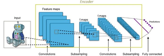
CNNs in encoders
For convolutional neural networks CNNs, the input image is converted to a more compact representation (typically a 1000-dimensional first-order tensor in ImageNet). This tight expression is used to classify the input image. The encoder works in a similar way. It converts the input data into a very small and compact representation (encoded) containing enough information for the decoder to produce the desired output. The encoder is generally trained with the rest of the network and optimized by back propagation errors to generate useful special codes. For CNNs, it can be seen as a special encoder. The output of the 1000-dimensional code is the classifier used for classification.
The self-encoder is based on the idea that the encoder output is used as a special purpose for reconstructing its input.
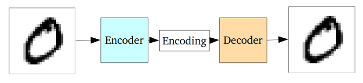
Standard self-encoder
The entire self-encoder neural network is often trained as a whole, and its loss function is defined as the mean squared error/cross-entropy between the reconstruction output and the original input as a reconstruction loss function to punish the network for generating a different output than the original input.
The code in the middle is used as the output of the hidden inter-layer links and its dimensions are much smaller than the output data. The encoder must selectively discard data, include as much relevant information as possible into the limited encoding, and intelligently remove irrelevant information. The decoder needs to learn as much as possible from the coding how to reconstruct the input image. Together they form the left and right arms of the encoder.
Problems with standard auto encoders
The standard self-encoder can learn to generate compact data representations and reconstruct the input data, but its application is extremely limited except for a few applications such as denoising autoencoders. The underlying reason is that the conversion of the input from the encoder into the implicit space is not continuous, making the interpolation and perturbation thereof difficult to complete.
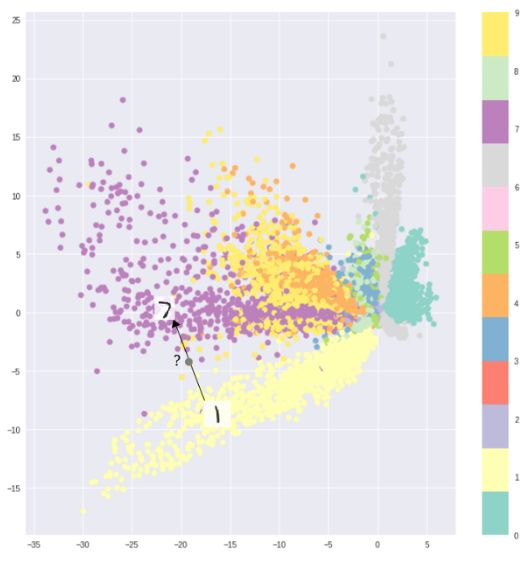
Interval between different classifications of MNIST data caused the encoder to continuously sample
For example, an auto-encoder trained using MNIST data sets maps data into 2D implicit spaces. There are obvious distances between the different categories. This makes it impossible for the decoder to decode the area existing between the categories with ease. If you don't want to just reproduce the input image, but want to randomly sample from the hidden space or make a certain change in the input image, then a continuous hidden space becomes indispensable.
If the implicit space is not contiguous, the decoder generates non-real output after sampling in different categories of intermediate gaps. Because the decoder does not know how to cover a blank area, it has never seen a sample in this area during training.
Variational self-encoder
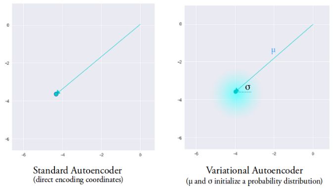
The variational self-encoder has completely different characteristics from the standard self-encoder, and its implicit space is designed to be continuously distributed for random sampling and interpolation, which makes it an efficient generation model. It does this in a very unique way. Instead of outputting a previous n-dimensional vector, the encoder outputs two n-dimensional vectors: the mean vector μ and the standard deviation vector σ, respectively.
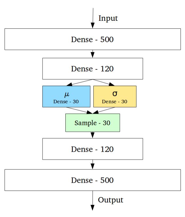
Then by sampling the mean and variance as μ and σ, the random variable Xi is obtained. After n samples, the n-dimensional sampled result is formed as the coded output and sent to the subsequent decoder.
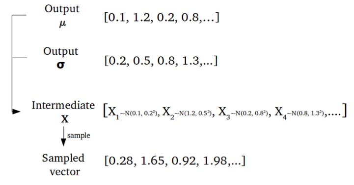
Randomly generated code vector
This random generation means that even for the same input of mean and variance, the actual encoding will produce different encoding results due to the difference of each sampling. The mean vector controls the center of the encoded input, while the standard deviation controls the size of this area (the range over which the encoding can change from the mean).
The code obtained through sampling can be any position in this area. The decoder learns not only the representation of a single point in the hidden space but the coded representation of the point within the entire neighborhood. This allows the decoder not only to decode a single specific code in the hidden space, but also to decode the code that changes to a certain extent, and this is because the decoder is trained by a certain degree of change in coding.
The resulting model is now exposed to a certain degree of localized change coding, making similar samples in the implicit space smooth at the local scale. Ideally, dissimilar samples have some overlap in the implicit space, making it possible to interpolate between different classes. However, there is still a problem with this method. We cannot give restrictions on the values ​​of μ and σ. This will cause the average value of the encoder to learn in different categories to be very different, and separate the clusters between them. Minimizing σ does not make the same sample much different. This allows the decoder to efficiently reconstruct from training data.
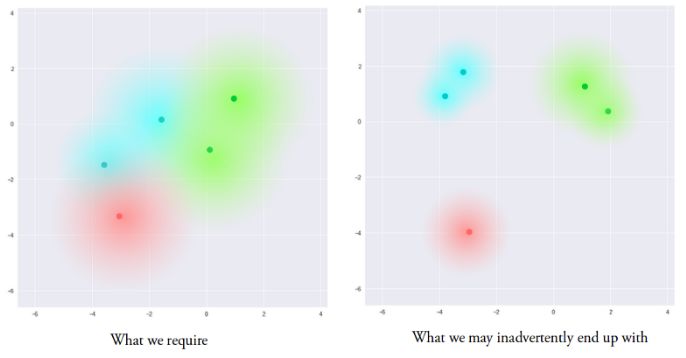
We want to get codes that are as close to each other but still have a certain distance in order to interpolate and recreate new samples in the hidden space. In order to achieve the required coding, Kullback-Leibler divergence (KL divergence) is introduced in the loss function. KL divergence describes the degree of divergence between two probability distributions. Minimizing KL divergence here means that the parameters (μ, σ) of the optimal probability distribution are as close as possible to the target distribution.
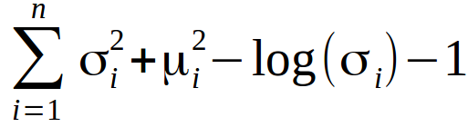
For VAE, the KL loss function is the divergence sum of all the elements Xi in the X (μi, σi2) and the standard normal distribution.
This loss function will encourage all codes to be distributed around the center of the hidden layer while penalizing the behavior of different classes being clustered into separate regions. The codes resulting from the pure KL divergence loss are randomly distributed in the center of the hidden space. However, decoders from these nonsense expressions cannot decode meaningful information.
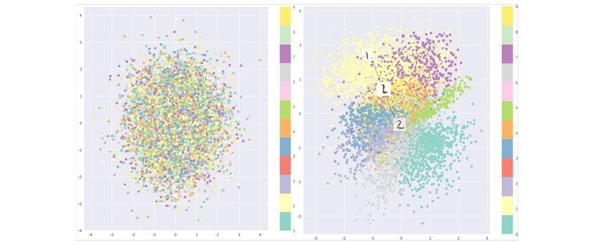
Pure KL divergence optimized implicit space (left), combined with reconstruction loss optimized implicit space
This is a combination of KL loss and reconstruction losses. This maintains the same category of hidden space points in the local area, while all points in the global scope are also compactly compressed into consecutive hidden spaces. This result is obtained by reconstructing the balance of the lost clustering behavior and the tightly distributed behavior of KL loss, thus forming an implicit spatial distribution that can be decoded by the decoder. This means that you can sample randomly and interpolate smoothly in the implicit space. The result is a controllable decoder that generates meaningful, valid results.
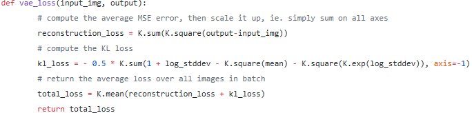
The final loss function
Vector operation
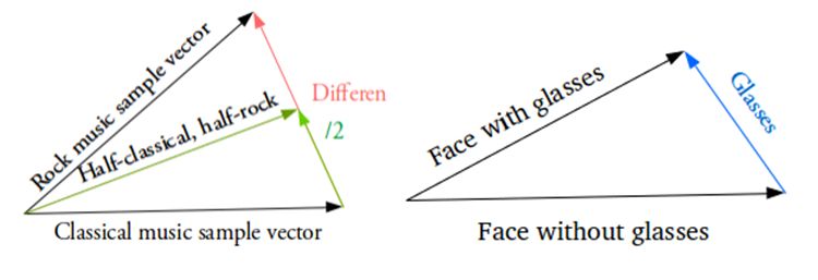
So how do we get smooth interpolation in implicit space now? This is mainly achieved by vector operations in the implicit space.
For example, if you want to get a new sample between two samples, then you only need to calculate the difference between their mean vectors and add half of them to the original vector. Finally, the results obtained can be sent to the decoder. What about special features such as how to generate glasses? Then find the samples with glasses and no glasses, and get the difference between their vectors in the hidden space of the encoder. This shows the characteristics of glasses. Adding this new "glasses" vector to any face vector and decoding it will result in a human face wearing glasses.
Outlook
For variational self-encoding, a variety of improved algorithms have emerged. You can add, replace standard full-connect codecs and replace them with convolutional networks. Someone used it to generate various face and famous MNIST change data.
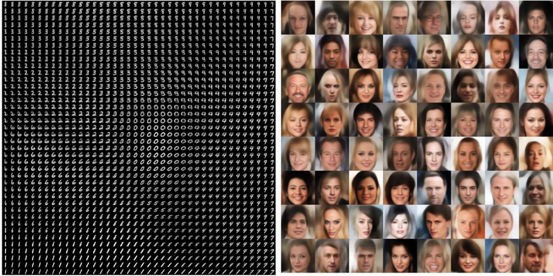
Even LSTM training codecs can be used to train time-series discrete data to generate sequence samples such as text and music. It can even imitate human sketches.
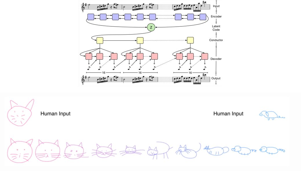
VAE is very adaptable to a wide variety of data, whether sequenced or non-sequential, continuous or discrete, labeled or unlabeled data are powerful generating tools. Look forward to seeing more unique applications in the future.
Paperlike Screen Protector For IPad
Paperlike Screen Protector,iPad Paperlike Screen Protector,Paperlike Screen Protector iPad
Shenzhen Jianjiantong Technology Co., Ltd. , https://www.jjtbackskin.com