
COMSOL Multiphysics® offers several different turbulence problem solving formulas: L-VEL, algebraic yPlus, Spalart-Allmaras, k-ε, k-ω, low Reynolds number k-ε, SST, and v2-f turbulence models. All these formulae can be called in the "CFD module", L-VEL, algebraic yPlus, k-ε and low Reynolds number k-ε are available in the "heat transfer module". This article briefly explains why we use these different turbulence models, how to choose from them, and how to use them effectively.
Turbulence Simulation Introduction
Let's start with the fluid flow on the plate, as shown in the figure below. The uniform velocity fluid contacts the leading edge of the plate and begins to form a laminar boundary layer. The flow in the area is easily predictable. After a certain distance, small chaotic oscillations begin to appear in the boundary layer, and the flow begins to turn into turbulent flow, and eventually completely turns into turbulent flow.
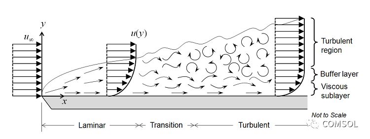
Transition between three regions can be achieved by Reynolds number 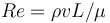


In the laminar flow region, fluid flow can be fully predicted by solving the steady-state Navier-Stokes equation, where the velocity and pressure fields are predicted. We can assume that the speed field does not change over time. The Blasius boundary layer model is one such example. When the flow starts to turn into a turbulent flow, even if the flow rate of the inlet does not change with time, chaotic oscillations may occur in the flow, and therefore it cannot be assumed that the flow does not change with time. In this case, the transient Navier-Stokes equation needs to be solved, and the grid used should also be fine enough to resolve the size of the smallest eddy current in the flow. The cylindrical flow model demonstrates such a situation. Both steady state and transient laminar flow problems can be solved with the COMSOL Multiphysics basic module without any additional modules.
With the increase of the flow rate and thus the Reynolds number, small eddy currents appear in the flow field. The spatial and temporal scales of the oscillations become very short, which makes it impossible to perform numerical analysis on them using the Navier-Stokes equations. In this flow pattern, we can use the Reynolds-averaged Navier-Stokes (RANS) equation, which is based on observations of the flow field (u) over time, including local small oscillations (u'), which can be treated as time-averaged terms ( U). For equations and two-equation models, we add turbulent variables by introducing other equations, such as turbulent kinetic energy (k in the k-ε and k-ω formulas).
In the algebraic model, an algebraic equation that depends on the velocity field (in some cases, the distance from the wall) is introduced to describe the turbulence intensity. The vortex viscosity, which increases the viscosity of the fluid molecules, is then calculated based on an estimate of the turbulent variables. The momentum transmitted by the small vortex turns into viscous transportation. In addition to the viscous underlayer near the solid walls, turbulent flow dissipation usually dominates the viscous dissipation throughout. Here, turbulence models (such as low Reynolds number models) must continually reduce turbulence levels. Or, you must use the wall function to calculate the new boundary condition.
Low Reynolds number model
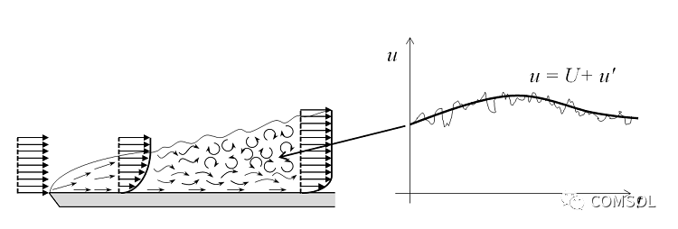
The term “low Reynolds number model†sounds contradictory, because if the Reynolds number is high enough, the flow can only be turbulent. The term “low Reynolds number†does not refer to global flow, but refers to the near-wall region dominated by the viscous effect; that is, the sticky bottom layer in the above figure. When the distance from the wall is close to zero, the low Reynolds number model can correctly reproduce the extreme behavior of different flows. Therefore, the low Reynolds number model must—for example—predict k~y2 as y→0. The correct extreme behavior means that the turbulence model can be used to simulate the entire boundary layer, including the adhesive bottom layer and the buffer layer.
Most ω-based models are low Reynolds number models. However, the standard k-ε model and other common k-ε models are not low Reynolds number models. However, some of these models can exhibit the correct limit behavior by adding so-called damping functions. This model is therefore called the low Reynolds number k-ε model.
Low Reynolds number models can often accurately describe the boundary layer. However, sharp gradients in the near wall require very high grid resolution, and high precision creates high computational costs. This is why alternative methods are often used in industrial applications to simulate near-wall flow.
Wall function
Turbulent flow near a flat wall can be divided into four areas. At the wall surface, the fluid velocity is 0, and for a thin layer above it, the fluid velocity and the distance from the wall surface change linearly. This area is called the adhesive bottom layer, or the laminar bottom layer. The area away from the wall is called the buffer layer. In the buffer zone, turbulent stress began to dominate the substitution of viscous stress, and the flow eventually turned into a turbulent flow in one zone, and the average flow velocity was related to the logarithm of the distance from the wall. This area is called the logarithmic region. In areas farther from the wall, the flow turns into a free-flow area. The adhesive and buffer layers are very thin if the distance to the bottom of the buffer is 

The RANS model can be used to calculate the flow field in all four regions. However, due to the very small thickness of the buffer layer, using an approximation in this area can be very helpful. The wall function ignores the buffer flow field and parses the non-zero flow velocity at the calculated wall surface. By using the wall function formula, you can assume an analytical solution for the flow in the viscous layer, greatly reducing the computational requirements of the resulting model. This is a very practical method for many practical engineering applications.

If the level of accuracy you require is higher than what the wall function formula can provide, consider a turbulence model that can solve the entire flow pattern (similar to the flow pattern in the low Reynolds number model above). For example, you may want to calculate lift and drag on an object, or calculate heat transfer between a fluid and a wall.
Automatic wall treatment
The automatic wall treatment function combines the advantages of the wall function and the low Reynolds number model. The automatic wall processing function adapts the formula to the grid available in the model, allowing you to gain both robustness and accuracy. For example, for a roughened boundary layer mesh, this function will use a robust wall function formula. However, for dense boundary layer meshes, the automatic wall processing function uses a low Reynolds number formula to completely decompose the velocity distribution into walls.
From the low Reynolds number formula to the wall function formula is a smooth transition. The COMSOL software mixes the two formulas in the boundary element. Then, the software calculates the distance (dimensionless lift distance) between the grid point of the boundary element and the wall surface. Then apply the formula combination to the boundary conditions.
In addition to the k-ε model, all turbulence models of COMSOL Multiphysics support the automatic wall processing function. This means that low Reynolds number models are also suitable for industrial applications, and their low Reynolds number modeling capabilities can only be invoked when the grid is fine enough.
About various turbulence models
The use of wall functions in these eight RANS turbulence models, the number of additional variables solved, and the meaning of the variables are all different. All of these models enhance the Navier-Stokes equations with additional turbulent viscosity terms, but their calculation methods are different.
L-VEL and yPlus
The L-VEL and yPlus algebraic turbulence models calculate turbulent viscosity based only on the local flow velocity and distance from the nearest wall; they do not solve additive variables. These models solve the flow everywhere and are robust in all eight models and have the lowest computational strength. Although they are the least accurate models, they are a good approximation to internal flow, especially in electronic cooling applications.
Spalart-Allmaras
The Spalart-Allmaras model adds an additional non-attenuating kinematic eddy viscosity variable. It is a low Reynolds number model that solves the entire flow field within a solid wall. The model was originally developed for aerodynamic applications, with the advantages of being relatively robust and requiring low resolution. From experience, the model does not accurately calculate the shear flow, the separation flow, or the field that attenuates the turbulence. Its advantage lies in its stability and good convergence.
K-ε
The k-ε model solves two variables: the æ¹ flow energy k and the æ¹ flow energy dissipation rate ε (epsilon). This model uses a wall function and therefore does not simulate the flow in the buffer. Since the k-ε model has a good convergence rate and relatively low memory requirements, it is popular in many industrial applications. However, it does not very accurately calculate the flow field in the flow or jet with an overpressure gradient and a strong curvature. It does a good job of solving external flow problems around complex geometries. For example, the k-ε model can be used to solve the airflow around a bluff body.
The turbulence models listed below are all more nonlinear than the k-ε model. Unless good initial guess values ​​are available, they are often difficult to converge. The k-ε model can be used to provide a good initial guess. Use the k-ε model to solve the model and then use the new Turbulence Interface function in COMSOL Multiphysics Version 5.3 "CFD Module".
K-ω
The k-ω model is similar to the k-ε model, but it solves the specific rate ω (omega) of kinetic energy dissipation. It is a low Reynolds number model but can be used in conjunction with a wall function. It is more nonlinear than the k-ε model, and therefore it is more difficult to converge and is quite sensitive to the initial guess of the solution. In many cases where the k-ε model is not accurate enough, the k-ω model can be very helpful, such as the internal flow, the flow showing strong curvature, the separation flow, and the jet. The flow through the elbow is a good example of internal flow.
Low Reynolds number k-ε
The low Reynolds number k-ε is similar to the k-ε model but no wall function is used. It solves the flow at each location, is a reasonable complement to k-ε, has the same advantages as the latter, but usually requires a denser grid; its low Reynolds number property not only appears on the wall but in each At work, turbulence decays. In some cases, it is recommended to first calculate a good initial condition using the k-ε model, and then use it to solve the low Reynolds number k-ε model. Another method is to use the automatic wall processing function. First, a roughened boundary layer mesh is used to obtain the wall function, and then the boundary layer at the desired wall surface is refined to obtain a low Reynolds number model.
The low Reynolds number k-ε model can calculate the lift and drag forces, and the heat flux modeling accuracy is much greater than the k-ε model. In many cases, it demonstrated excellent predictive separation and reattachment capabilities.
SST
Finally, the SST model combines the k-ε in free flow and the near-wall k-ω model. It is a low Reynolds number model and is a "universal" model in industrial applications. In terms of resolution requirements, the model is similar to the k-ω model and the low Reynolds number model, but its formula eliminates some of the weaknesses shown by the k-ω model and the k-ε model. In the example model, the flow over the NACA 0012 wing surface was solved by the SST model and the results were in agreement with the experimental data.
V2-f
Near the wall boundary, the velocity pulsation in the parallel direction is usually much larger than the direction perpendicular to the wall surface. Velocity pulsations are considered anisotropic. In areas far from the wall, the pulsations in all directions are the same, and the velocity pulsation becomes isotropic.
In addition to the two equations that describe the turbulent kinetic energy (k) and the dissipation rate (ε), respectively, the v2-f turbulence model uses two new equations to describe the turbulent intensity anisotropy in the turbulent boundary layer. The first equation describes the transfer of turbulent velocity pulsations perpendicular to the streamline. The second equation explains the non-local effect, such as the wall-induced damping of the redistribution of turbulent kinetic energy between vertical and parallel directions.
You should use this model to describe closed flows on surfaces such as cyclonic modeling.
Grid meshing considerations
Regardless of laminar or turbulent flow, the computational strength of solving any fluid flow problem is high. Not only does it require a relatively fine mesh, but it also requires the solution of many variables. Ideally, you should use high-speed computers with large memory to solve such problems. Even then, the simulation of large-scale 3D models may take hours or even days. Therefore, we want to use a grid that is as simple as possible, but can get all the details in the flow.
Now look at the graph at the top, and we can observe that for slabs (and most of the flow problems), the velocity field changes quite slowly in the direction of the wall tangent, but it changes quickly in the normal direction, especially considering the buffer layer area Case. This observation also encourages the use of boundary layer meshes. The boundary layer mesh (when using a physics field to control the mesh, the default mesh type for the wall) inserts an elongated two-dimensional rectangle or a three-dimensional triangular prism on the wall surface. The unit with a larger height and width can resolve the flow rate change in the direction of the boundary method very well, while reducing the number of calculation points in the boundary tangential direction.
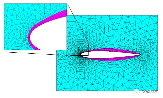
The boundary layer mesh (purple) around the wing in the 2D mesh, and the surrounding triangle mesh (cyan).
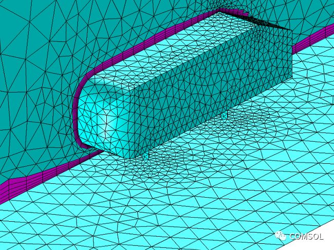
The boundary layer mesh (purple) surrounding the bluff body in the three-dimensional body mesh, and the surrounding tetrahedral mesh (cyan).
Turbulence Model Calculation Results
When using these turbulence models to solve flow simulations, you will want to verify that the solution is accurate. Of course, just like any other finite element model, you can simply use a more and more refined mesh to re-simulate and see how the solution changes with the degree of refinement of the mesh. Once the solution has not changed within your acceptable range, your simulation is considered to converge relative to the grid. But when simulating turbulence, there are other values ​​that need to be checked.
When using wall function formulas, you will want to check the dimensionless wall resolution (the drawing is generated by default). This value is used to determine the start and end of the computational domain of the boundary layer, and should not be too large. If wall resolution exceeds a few hundred, you should use a more refined boundary layer mesh in these areas. When using a wall function, the second variable that should be checked is the wall lift distance in units of length. This variable is related to the assumed thickness of the viscous layer and should be small relative to the surrounding geometry. If not, you should refine the grid of these areas.
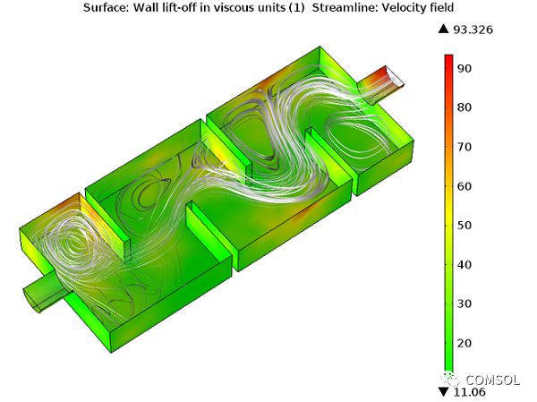
The dimensionless maximum wall lift distance is less than 100, so there is no need to refine the boundary layer mesh.
When using the automatic wall processing function to solve the low Reynolds number model, check the dimensionless distance to the center of the element (which will be generated by default). In algebraic models, this value should be the same magnitude in every place, and it should be less than 0.5 in the two-equation model and the v2-f model. If it is larger than this value, the mesh should be refined in these areas.
Ending message
This article describes the various turbulence models provided by COMSOL Multiphysics and when and why they are used. The real advantage of the software lies in the fact that when you want to couple fluid flow simulations with other physical fields, here are just a few examples, such as finding out the stress on a solar panel in a strong wind, simulating forced convection in a heat exchanger, or stirring Mass transfer in the device, etc.
Terminal Wires,Black Tinned Copper Terminal Wires,Bare Copper Terminal Wires,Tinned Copper Terminal Wires
Dongguan ZhiChuangXing Electronics Co., LTD , https://www.zcxelectronics.com