
Editor's Note: Six months ago, the Shanghai Jiaotong University Chen Tianqi team opened up the end-to-end IR stack tool TVM, which can help users optimize the Hardware configuration during the deep learning process, alleviating the insufficient performance of most current computer GPUs in the face of deep learning. . Recently, a student of the team, Zheng Mercy, brought new developments to the project. He used TVM for the ARM GPU, which is common on the mobile side, and improved the mobile device's ability to support deep learning.

The following is the translation of the original text:
As deep learning continues to advance, developers are increasingly demanding the deployment of neural networks on mobile devices. Similar to the previous attempts we have made on desktop GPUs, porting the deep learning framework to the mobile side requires two things: fast inference speed and reasonable power consumption. However, most of today's DL frameworks do not support mobile GPUs well because they differ greatly from desktop GPUs in architecture. In order to do deep learning on the mobile side, developers often have to do some special optimizations on the GPU, and this extra work also increases the pressure on the GPU.
TVM is an end-to-end IR stack that solves the problem of resource allocation during learning, making hardware optimization easy. In this article, we will show how to use TVM/NNVM to generate efficient kernels for ARM Mali GPUs and perform end-to-end compilation. In the test of the Mali-T860 MP4, our method was 1.4 times faster on the VGG-16 than the Arm Compute Library and 2.2 times faster on the MobileNet. These improvements are reflected in image processing and computation.
Mali Midgard GPU
Currently, the three most common graphics processors in the mobile space are Qualcomm's Adreno, UK PowerVR and ARM's embedded graphics processor Mali. Our test environment is the Firefly-RK3399 development board with the Mali-T860 MP4 GPU, so below we focus on the performance of the Mali T8xx.
Architecture
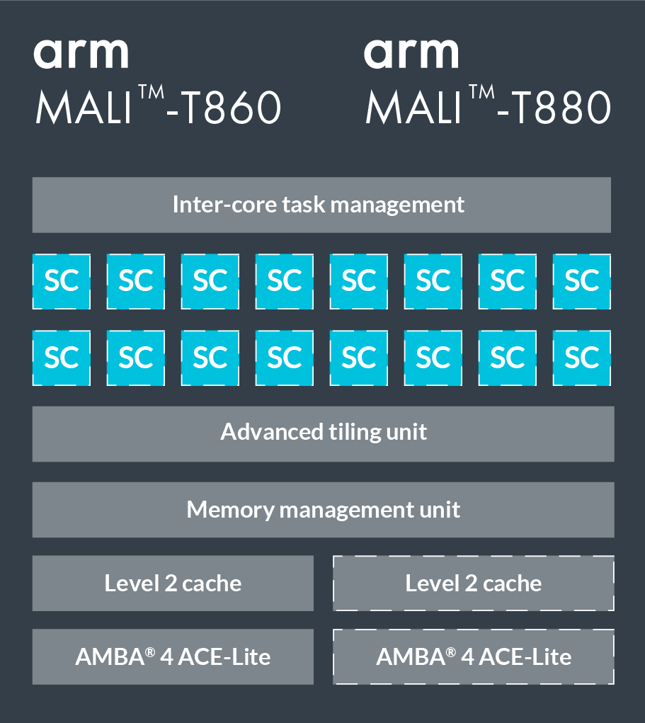
The T860 and T880 are two high-end GPUs in the Mali series. The following figure shows the specific configuration. They have 16 shader cores, each containing 2-3 computation pipelines, 1 load/store pipeline, and 1 texture pipeline (the Triple Pipeline architecture). The ALU (arithmetic logic unit) in the operation pipeline contains four 128-bit vector units and one scalar unit.
We write programs in OpenCL. When mapped to the OpenCL model, each shader core executes one or more workgroups, the upper limit of which is to execute 384 threads in parallel, usually one workgroup corresponds to one thread. The Mali series of GPUs use the VLIW architecture (long instruction set architecture), so each instruction contains multiple operations; at the same time, it also uses SIMD (single instruction stream multiple data streams), so most of the arithmetic operations can be executed simultaneously. Multiple data streams.
The difference between NVIDIA GPU and NVIDIA GPU
Before optimizing the GPU with TVM, let's take a look at the difference between Mali GPU and NVIDIA GPU:
NVIDIA GPU storage system architecture is generally divided into three levels of global memory, shared memory, and registers. In practice, we usually copy data to shared memory; while Mali GPU has only one unified global memory, it does not need to make a copy to improve performance. Because this memory is shared with the CPU, there is no need to copy between the CPU and the GPU;
The Mali Midgard GPU is based on SIMD design, so vector is needed. In NVIDIA CUDA, GPU parallel processing is implemented by SIMT, so it does not have such high requirements for vectors. It should be noted that the graphics processor of the Mali Bifrost architecture has newly added Quad based vectorization technology, which allows four threads to be executed together, and it does not need vectors.
Each thread in the Mali GPU has a separate program counter, warp size=1, so Branch Divergence is not a problem.
Optimization: Take the convolution layer as an example
Convolutional layers are at the heart of many deep neural networks and take up most of the computing resources. So let's take the convolutional layer as an example to talk about the optimization application of TVM in pack, tile, unroll, and vectorization.
Im2col+GEMM
Im2col is a common method of convolution calculation. It converts the problem into a matrix and then calls GEMM to complete the matrix multiplication. The advantage of this approach is that it is easy to combine with the highly optimized BLAS library, which has the disadvantage of consuming a lot of memory.
Spatial Packing
So we changed a method, first calculate the convolution, and then gradually apply optimization techniques. Take the convolution layer in VGG-16 as an example (as shown in the figure below), the batch size=1 of inference.

To provide a control group, we have listed the data for the Arm Compute Library.

Pack and tile are two common instructions for adjusting memory. The tile divides the data into slices, making each slice suitable for shared memory use; and pack re-lays the input matrix (memory alignment) so that we can read the data sequentially.
We used tile(tvm.compute) on the width of the input image and the CO dimension of the filter matrix:
# set tiling factor
VH = 1
VW = VC = 4
# get input shape
_, CI, IH, IW = data.shape
CO, CI, KH, KW = kernel.shape
TH = IH + 2 * H_PAD
TW = IW + 2 * W_PAD
# calc output shape
OH = (IH + 2*H_PAD - KH) // H_STR + 1
OW = (IW + 2*W_PAD - KW) // W_STR + 1
# data shape after packing
Dvshape = (N, TH // (VH*H_STRIDE), TW // (VW*W_STRIDE), CI, VH*H_STRIDE+HCAT, VW*W_STRIDE+WCAT)
#芯 shape after packing
Kvshape = (CO // VC, CI, KH, KW, VC)
Ovshape = (N, CO // VC, OH // VH, OW // VW, VH, VW, VC)
Oshape = (N, CO, OH, OW)
# define packing
Data_vec = tvm.compute(dvshape, lambda n, h, w, ci, vh, vw:
Data_pad[n][ci][h*VH*H_STRIDE+vh][w*VW*W_STRIDE+vw], name='data_vec')
Kernel_vec = tvm.compute(kvshape, lambda co, ci, kh, kw, vc:
Kernel[co*VC+vc][ci][kh][kw], name='kernel_vec')
# define convolution
Ci = tvm.reduce_axis((0, CI), name='ci')
Kh = tvm.reduce_axis((0, KH), name='kh')
Kw = tvm.reduce_axis((0, KW), name='kw')
Conv = tvm.compute(ovshape, lambda n, co, h, w, vh, vw, vc:
Tvm.sum(data_vec[n, h, w, ci, vh*H_STRIDE+kh, vw*W_STRIDE+kw].astype(out_dtype) *
Kernel_vec[co, ci, kh, kw, vc].astype(out_dtype),
Axis=[ci, kh, kw]), name='conv')
# unpack to correct layout
Output = tvm.compute(oshape, lambda n, co, h, w:
Conv[n][co//VC][h/VH][w//VW][h%VH][w%VW][co%VC],
Name='output_unpack', tag='direct_conv_output')
Check the defined IR with the following command:
Print(tvm.lower(s, [data, kernel, output], simple_mode=True))
Select the part of the convolution:
Produc conv {
For (co, 0, 64) {
For (h, 0, 56) {
For (w, 0, 14) {
For (vw.init, 0, 4) {
For (vc.init, 0, 4) {
Conv[(((((((co)))))))))))))))))))))))))))))))))))
}
}
For (ci, 0, 256) {
For (kh, 0, 3) {
For (kw, 0, 3) {
For (vw, 0, 4) {
For (vc, 0, 4) {
Conv[(((((((((((((((((((((((((((((((((((((((((( 56) + h)*14) + w)*4) + vw)*4) + vc)] + (data_vec[(((((((((*()))))) *3) + kh)*6) + kw) + vw)]*kernel_vec[(((((((co))))))))))))))))))))))) Vc)]))
}
}
}
}
}
}
}
}
}
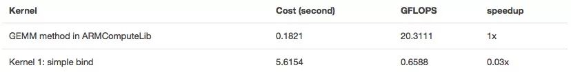
Kernel 1: binding thread
In TVM, we first calculate and then schedule, which facilitates separation of algorithms and implementation details.
As the code shows, we simply map the axes axis to the GPU thread and then run the code on the Mali GPU.
# helper function for binding thread
Def tile_and_bind3d(s, tensor, z, y, x, z_factor=2, y_factor=None, x_factor=None):
""" tile and bind 3d """
Y_factor = y_factor or z_factor
X_factor = x_factor or y_factor
Zo, zi = s[tensor].split(z, z_factor)
Yo, yi = s[tensor].split(y, y_factor)
Xo, xi = s[tensor].split(x, x_factor)
s[tensor].bind(zo, tvm.thread_axis("blockIdx.z"))
s[tensor].bind(zi, tvm.thread_axis("threadIdx.z"))
s[tensor].bind(yo, tvm.thread_axis("blockIdx.y"))
s[tensor].bind(yi, tvm.thread_axis("threadIdx.y"))
s[tensor].bind(xo, tvm.thread_axis("blockIdx.x"))
s[tensor].bind(xi, tvm.thread_axis("threadIdx.x"))
# set tunable parameter
Num_thread = 8
# schedule data packing
_, h, w, ci, vh, vw = s[data_vec].op.axis
Tile_and_bind3d(s, data_vec, h, w, ci, 1)
# schedule kernel packing
Co, ci, kh, kw, vc = s[kernel_vec].op.axis
Tile_and_bind(s, kernel_vec, co, ci, 1)
# schedule conv
_, c, h, w, vh, vw, vc = s[conv].op.axis
Kc, kh, kw = s[conv].op.reduce_axis
s[conv].reorder(_, c, h, w, vh, kc, kh, kw, vw, vc)
Tile_and_bind3d(s, conv, c, h, w, num_thread, 1, 1)
_, co, oh, ow = s[output].op.axis
Tile_and_bind3d(s, output, co, oh, ow, num_thread, 1, 1)
Even with this schedule, we can now run the code, but its performance requirements are quite scary.
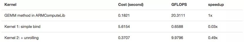
Kernel 2: unroll
Loop unrolling is a commonly used optimization method that reduces the overhead of the loop itself by reducing loop control instructions. It also amortizes some branch overheads by eliminating branches and some code that manages the inductive variables. It also masks the latency of reading memory. In TVM, you can call s.unroll(axis) to implement loop unrolling.
# set tunable parameter
Num_thread = 8
# schedule data packing
_, h, w, ci, vh, vw = s[data_vec].op.axis
Tile_and_bind3d(s, data_vec, h, w, ci, 1)
"""!! ADD UNROLL HERE !!"""
s[data_vec].unroll(vw)
# schedule kernel packing
Co, ci, kh, kw, vc = s[kernel_vec].op.axis
Tile_and_bind(s, kernel_vec, co, ci, 1)
"""!! ADD UNROLL HERE !!"""
s[kernel_vec].unroll(kh)
s[kernel_vec].unroll(kw)
s[kernel_vec].unroll(vc)
# schedule conv
_, c, h, w, vh, vw, vc = s[conv].op.axis
Kc, kh, kw = s[conv].op.reduce_axis
s[conv].reorder(_, c, h, w, vh, kc, kh, kw, vw, vc)
Tile_and_bind3d(s, conv, c, h, w, num_thread, 1, 1)
"""!! ADD UNROLL HERE !!"""
s[conv].unroll(kh)
s[conv].unroll(kw)
s[conv].unroll(vw)
s[conv].unroll(vc)
_, co, oh, ow = s[output].op.axis
Tile_and_bind3d(s, output, co, oh, ow, num_thread, 1, 1)
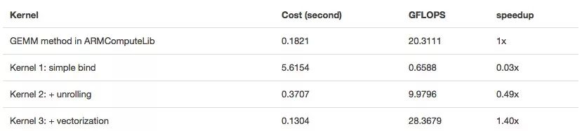
Kernel 3: vectorization
As mentioned earlier, in order to achieve optimal performance on the Mali GPU, we also need to convert the numbers into vectors.
# set tunable parameter
Num_thread = 8
# schedule data packing
_, h, w, ci, vh, vw = s[data_vec].op.axis
Tile_and_bind3d(s, data_vec, h, w, ci, 1)
# unroll
s[data_vec].unroll(vw)
# schedule kernel packing
Co, ci, kh, kw, vc = s[kernel_vec].op.axis
Tile_and_bind(s, kernel_vec, co, ci, 1)
# unroll
s[kernel_vec].unroll(kh)
s[kernel_vec].unroll(kw)
"""!! VECTORIZE HERE !!"""
s[kernel_vec].vectorize(vc)
# schedule conv
_, c, h, w, vh, vw, vc = s[conv].op.axis
Kc, kh, kw = s[conv].op.reduce_axis
s[conv].reorder(_, c, h, w, vh, kc, kh, kw, vw, vc)
Tile_and_bind3d(s, conv, c, h, w, num_thread, 1, 1)
# unroll
s[conv].unroll(kh)
s[conv].unroll(kw)
s[conv].unroll(vw)
"""!! VECTORIZE HERE !!"""
s[conv].vectorize(vc)
_, co, oh, ow = s[output].op.axis
Tile_and_bind3d(s, output, co, oh, ow, num_thread, 1, 1)
How to set tunable parameters
Some of the tunable parameters mentioned above can be calculated, such as vector vc, if it is float32, |vc|=128/32=4; if it is float16, it is 128/16=8.
However, due to the long running time, we often cannot determine the best value. TVM uses grid search, so if we use Python instead of OpenCL, we can quickly find the best value.
End-to-end Benchmark
In this section, we compare the comprehensive performance of some popular deep neural networks on different backends. The test environment is:
Firefly-RK3399 4G
CPU: dual-core Cortex-A72 + quad-core Cortex-A53
GPU: Mali-T860MP4
ArmComputeLibrary : v17.12
MXNet: v1.0.1
Openblas: v0.2.18
We use NNVM and TVM for end-to-end compilation.
performance
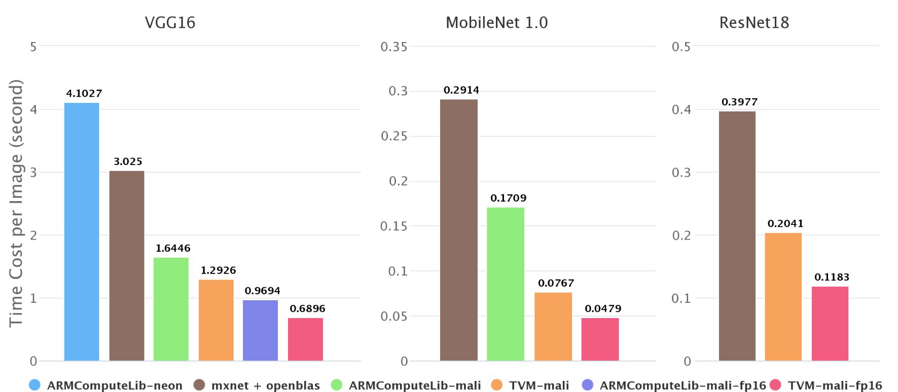
Inference speed of different backends on ImageNet
As shown in the above figure, we tested the inference speed of the mobile neural network in ImageNet and found that on the Firefly-RK3399, the Mali GPU can be 2-4 times faster than the 6-core big.LITTLE CPU. Our end-to-end compilation speed is better than Arm. Compute Library is 1.4-2.2 times faster. In the Arm Compute Library, we compared the convolution with GEMM and directly calculated the convolution, and found that the former is always faster, so only the results of the GEMM method are shown in the figure.
There are also some missing data in the above figure, such as the second picture does not contain resnet18 on the Arm Compute Library. This is because the arm runtime of the Arm Compute Library does not currently support jump connections, and Neon's implementation performance is not very good. This also reflects the advantages of the NNVM software stack.
Semi-precision performance
Deep neural networks do not require high precision, especially for mobile devices where computing resources are stretched. Reduced accuracy can speed up the inference speed of neural networks. We also calculated the half-precision floating point numbers on the Mali GPU.
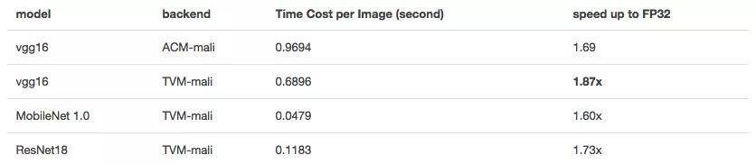
Inference speed of FP16 on mageNet
In theory, FP16 can achieve double-peak calculations and halve the memory consumption, thus doubling the speed. But if it involves longer vectorization and fine-tuning of certain parameters, it also requires a good input form.
Arcade Game Console,game console,video game consoles,arcade games console
Guangzhou Ruihong Electronic Technology CO.,Ltd , https://www.callegame.com