
(1) A framework to understand the optimization algorithm
When it comes to optimization algorithms, the entry level must learn from SGD. The old driver will tell you that AdaGrad / AdaDelta is better, or Adam is directly brainless. But look at the latest paper in academia, but find a lot of gods. Still using the entry-level SGD, add up to Momentum or Nesterov, and often black Adam. Why?"
There are a group of alchemists in the machine learning world. Their daily routine is:
Bring the medicinal materials (data), set up the gossip furnace (model), and point the six-flavored real fire (optimization algorithm), then shake the Pufan and wait for the medicinal herbs to come out.
However, all the cooks know that the same ingredients, the same recipes, but the heat is not the same, the taste is very different. The fire is small, the fire is big and easy to paste, and the fire is uneven.
The same is true for machine learning. The choice of model optimization algorithm is directly related to the performance of the final model. Sometimes the effect is not good, not necessarily the problem of the feature or the problem of the model design, it is probably the problem of the optimization algorithm.
When it comes to optimization algorithms, the entry level must learn from SGD, and the old driver will tell you that AdaGrad / AdaDelta is better, or Adam is directly brainless. But look at the latest papers in academia, but found that the great gods are still using the entry-level SGD, plus a maximum of Momentum or Nesterov, and often black Adam. For example, a paper by UC Berkeley wrote in Conclusion:
Despite the fact that our experimental evidence demonstrates that adaptive methods are not advantages for machine learning, the Adam algorithm remains incredibly popular. We are not sure exactly as to why ......
Helplessness and sorrow and grief are beyond words.
Why is this? Is it true that it is faint?
▌01 A framework review optimization algorithm
First let's review the various optimization algorithms.
The deep learning optimization algorithm has experienced the development process of SGD -> SGDM -> NAG -> AdaGrad -> AdaDelta -> Adam -> Nadam. Google can see a lot of tutorial articles at a glance, telling you in detail how these algorithms evolved step by step. Here, we change the idea, use a framework to sort through all the optimization algorithms, and make a more high-level comparison.
Optimization algorithm general framework
First define: parameters to be optimized: w, objective function: f(w), initial learning rate α. Then, iterative optimization begins. At each epoch t:
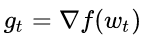
1. Calculate the gradient of the objective function with respect to the current parameters:
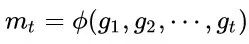
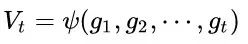
2. Calculate first-order momentum and second-order momentum from historical gradients:
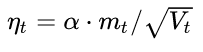
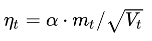
3. Calculate the falling gradient at the current moment:
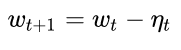
4. Update according to the descending gradient:
With this framework in place, you can easily design your own optimization algorithms.
We took this frame and took photos of the realities of various mysterious optimization algorithms. Steps 3 and 4 are consistent for each algorithm, and the main differences are reflected in 1 and 2.
▌02 Optimization algorithm for fixed learning rate
SGD
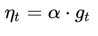
Let's look at SGD first. SGD has no concept of momentum, that is:
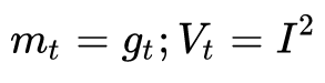
Substitute step 3, you can see that the descending gradient is the simplest
The biggest drawback of SGD is that it slows down and may continue to oscillate on both sides of the gully, staying at a local optimum.
SGD with Momentum
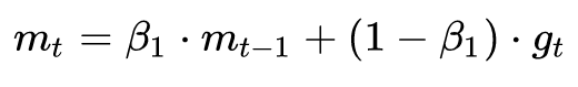
In order to suppress the oscillation of SGD, SGDM believes that the gradient descent process can add inertia. When going downhill, if you find it is a steep slope, then use inertia to run faster. The full name of SGDM is SGD with momentum, which introduces first-order momentum on the basis of SGD:
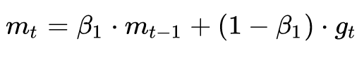
The first-order momentum is the exponential moving average of the gradient direction at each moment, which is approximately equal to the average of the gradient vector sums of the nearest 1/(1-β1) moments.
That is to say, the direction of d at the time t is determined not only by the gradient direction of the current point but also by the direction of the drop accumulated before. The empirical value of β1 is 0.9, which means that the downward direction is mainly the cumulative downward direction and slightly biased toward the current direction. Imagine a car turning on a highway, a slight bias at the high speed forward, and a sharp turn is going to happen.
SGD with Nesterov Acceleration
Another problem with SGD is that it is trapped inside a locally optimal gully. Imagine that you are walking into a basin, surrounded by slightly higher hills. If you don't think there is a downhill direction, you can only stay here. But if you climb to the highlands, you will find that the world outside is still very broad. Therefore, we can't stay in the current position to observe the direction of the future, but to take a step forward, look at one step, and look farther.
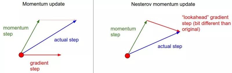
(source: http://cs231n.github.io/neural-networks-3)
This method, also known as NEGA, is Nesterov Accelerated Gradient, which is a further improvement based on SGD and SGD-M. The improvement lies in step 1. We know that the main direction of decline at time t is determined by the cumulative momentum, and the direction of the gradient is not counted. It is better to look at the current gradient direction. If you take a step with the cumulative momentum, then how do you go? . Therefore, in step 1, the NAG does not calculate the gradient direction of the current position, but calculates the downward direction at that time if one step is taken according to the cumulative momentum:
Then use the gradient direction of the next point, combined with the historical cumulative momentum, to calculate the cumulative momentum at the current moment in step 2.
▌03 Adaptive learning rate optimization algorithm
We have not used second-order momentum before. The emergence of second-order momentum means the arrival of the era of "adaptive learning rate" optimization algorithm. SGD and its variants update each parameter with the same learning rate, but deep neural networks often contain a large number of parameters that are not always available (think large-scale embedding).
For frequently updated parameters, we have accumulated a lot of knowledge about it, do not want to be too much affected by a single sample, and hope that the learning rate is slower; for the parameters that are updated occasionally, we know too little information, hoping to get from every accident The sample that appears appears to learn more, that is, the learning rate is larger.
AdaGrad
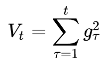
How to measure the historical update frequency? That is the second-order momentum—the sum of the squares of all gradient values ​​to date in this dimension:
Let us review the descending gradient in step 3:
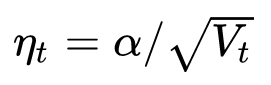
It can be seen that the actual learning rate at this time is  became
 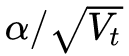 . Generally, in order to avoid the denominator being 0, a small smoothing term is added to the denominator. therefore
  It is constant greater than 0, and the more frequent the parameter update, the larger the second-order momentum, the smaller the learning rate.
This method performs very well in sparse data scenarios. But there are also some problems: because It is monotonously increasing, which will cause the learning rate to monotonically decrease to 0, which may make the training process end prematurely, even if there is still data to learn the necessary knowledge.
AdaDelta / RMSProp
Since the learning rate of AdaGrad monotonically decreasing is too radical, we consider a strategy to change the second-order momentum calculation method: not accumulating all historical gradients, but only focusing on the falling gradient of the window in the past period of time. This is the origin of Delta in the AdaDelta name.
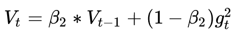
The idea of ​​modification is simple. As we mentioned earlier, the exponential moving average is about the average of the past period of time, so we use this method to calculate the second-order cumulative momentum:
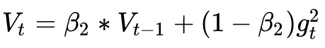
This avoids the problem that the second-order momentum continues to accumulate, leading to the early termination of the training process.
Adam
When it comes to it, the appearance of Adam and Nadam is natural – they are the masters of the aforementioned methods. We see that SGD-M adds first-order momentum to SGD, and AdaGrad and AdaDelta add second-order momentum to SGD. The use of both first-order momentum and second-order momentum is Adam's - Adaptive + Momentum.
First order momentum of SGD:
Plus the second-order momentum of AdaDelta:
The two most common hyperparameters in the optimization algorithm 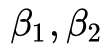 It is here, the former controls the first-order momentum, and the latter controls the second-order momentum.
Nadam
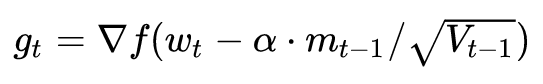
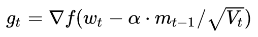
Finally, Nadam. We said that Adam is a great master, but it actually misses Nesterov, can this be tolerated? It must be added - just follow the step 1 of the NAG to calculate the gradient:

This is Nesterov + Adam = Nadam.
Having said that, it is probably possible to understand why Adam / Nadam is currently the most mainstream and best-used algorithm. There is no brain for Adam/Nadam, the convergence speed is dripping, and the effect is also the lever drop.
Then why is Adam still swaying and being scorned by the academic community? Is it just for sending paper water?
(2) Two sins of Adam
"Generation researchers have been painstakingly trying to refine (xun) gold (mo) Dan (xing). In theory, the generation is better than one generation, and Adam/Nadam has reached its peak. Why? Do you still remember the original heart SGD?"
In the above, we use a framework to review the mainstream deep learning optimization algorithms. It can be seen that generation after generation of researchers can be said to be painstaking for us to refine (xun) good (hao) gold (mo) xing (xing). In theory, the generation is better than the first generation, Adam/Nadam has reached its peak, why do you still remember the original heart SGD?
Give a chestnut. Many years ago, photography was very far away from the general public. Ten years ago, the point-and-shoot camera became popular, and the tourists were almost one. After the emergence of smart phones, photography is going into thousands of households. The mobile phone is ready to shoot, and 20 million before and after, illuminate your beauty (hey, this is a mess). But professional photographers still like to use SLR, tirelessly adjust the aperture, shutter, ISO, white balance... a bunch of self-portrait party no care term. Advances in technology have made fool-like operations a good result, but in certain scenarios, to get the best results, you still need to understand the light, understand the structure, and understand the equipment.
The optimization algorithm is also the same. In the previous article, we used the same framework to get all kinds of algorithms in check. It can be seen that everyone is on the same path, but it is equivalent to increasing the active control of various learning rates on the basis of SGD. If you don't want to do fine tuning, then Adam is obviously the easiest to use directly.
But such a fool-like operation does not necessarily suit all occasions. If you can get a deeper understanding of the data, it is not surprising that researchers can more easily control the various parameters of the optimization iteration to achieve better results. After all, the fine-tuned parameters are better than the fool-like SGD, which is undoubtedly challenging the top researchers' alchemy experience!
Recently, a lot of paper opened up Adam, we simply look at what is being said:
▌04 Adam guilty one: may not converge
This is a paper in the anonymous review of ICLR 2018, one of the top conferences in the field of deep learning, "On the Convergence of Adam and Beyond", which explores the convergence of the Adam algorithm, and by way of illustration, Adam may in some cases Will not converge.
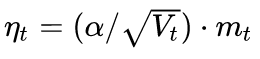
Recall the learning rates of the various optimization algorithms mentioned above:
Among them, SGD does not use second-order momentum, so the learning rate is constant (the learning rate attenuation strategy is adopted in the actual use process, so the learning rate is decremented). AdaGrad's second-order momentum is accumulating and monotonically increasing, so the learning rate is monotonically decreasing. Therefore, these two kinds of algorithms will make the learning rate decrease continuously, and finally converge to 0, and the model will also converge.
But AdaDelta and Adam are not. The second-order momentum is the accumulation in a fixed time window. As the time window changes, the data encountered may change greatly, making  It may be big or small, not monotonous. This may cause the learning rate to oscillate in the later stages of training, resulting in the model not being able to converge.
This article also gives a way to fix it. Since the learning rate in Adam is mainly controlled by the second-order momentum, in order to ensure the convergence of the algorithm, the change of the second-order momentum can be controlled to avoid fluctuations.

By modifying this way, it is guaranteed
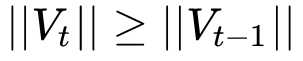
Thereby the learning rate is monotonically decreasing.
▌05 Adam guilty two: may miss the global optimal solution
Deep neural networks often contain a large number of parameters. In such a very high space, non-convex objective functions tend to rise and fall, with countless highlands and depressions. Some are peaks, and it is easy to cross them by introducing momentum; but some are plateaus, and they may not be able to find them many times, so they stopped training.
Previously, two articles on Arxiv talked about this issue.
The first one is the UC Berkeley article "The Marginal Value of Adaptive Gradient Methods in Machine Learning", which was mentioned in the previous article. As mentioned in the article, for the same optimization problem, different optimization algorithms may find different answers, but adaptive learning rate algorithms often find very poor solutions. They designed a specific data example. The adaptive learning rate algorithm may over-fitting the features that appeared in the previous period. It is difficult to correct the previous fitting effect when the features appear later. But the examples given in this article are extreme and may not necessarily appear in actual situations.
The other one is "Improving Generalization Performance by Switching from Adam to SGD" and has been experimentally verified. Tested on their CIFAR-10 dataset, Adam's convergence speed is faster than SGD, but the result of the final convergence is not as good as SGD. Their further experiments found that the learning rate of Adam in the late stage was too low, which affected the effective convergence. They tried to control the lower bound of Adam's learning rate and found that the effect was much better.
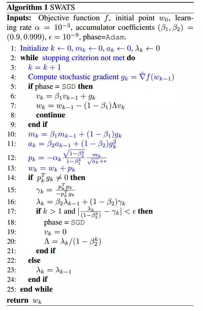
So they proposed a method to improve Adam: Adam used in the early stage, and enjoyed the advantage of Adam's fast convergence; later switched to SGD and slowly searched for the optimal solution. This method has also been used by researchers before, but mainly based on experience to choose the timing of switching and the learning rate after switching. This article fools this switching process, gives the timing of switching SGD, and the calculation method of learning rate. The effect looks good.
This algorithm is very interesting. We can talk about the next one. Here is an algorithm framework:
▌06 Should I use Adam or SGD?
So, when it comes to the present, is Adam good or SGD good? This may be a difficult thing to say in a word. Going to see the various papers in the academic conference, a lot of SGD, Adam is also a lot, there are many prefer AdaGrad or AdaDelta. It is possible that the researcher has tried each algorithm once, and which one works better. After all, the focus of paper is to highlight one's contribution in one aspect. Of course, other aspects are all-or-nothing. How can you lose in the details?
From the papers of these screaming Adams, most of them have constructed some more extreme examples to demonstrate the possibility of Adam's failure. These examples are generally too extreme, and may not necessarily be the case in practice, but this reminds us of the need for data to design algorithms. The evolution history of the optimization algorithm is based on the optimization of some assumptions about the data. If an algorithm is effective, it depends on whether your data meets the appetite of the algorithm.
The algorithm is beautiful, and the data is fundamental.
On the other hand, although Adam's stream has simplified the adjustment, it does not solve the problem once and for all. The default parameters are good, but they are not universal. Therefore, on the basis of fully understanding the data, it is still necessary to carry out sufficient adjustment experiments based on the data characteristics and algorithm characteristics.
Young, good alchemy.
(3) Selection and use strategies of optimization algorithms
“In the previous two articles, we used a framework to sort out the major optimization algorithms, and pointed out the possible problems of the adaptive learning rate optimization algorithm represented by Adam. So, how should we choose in practice? Introduce the combined strategy of Adam + SGD, and some useful tricks."
▌07 Core differences between different algorithms: the direction of decline
From the framework of the first article, we see that the core difference between different optimization algorithms is the downward direction of the third step:
In this equation, the first half is the actual learning rate (ie, the falling step size), and the second half is the actual falling direction. The falling direction of the SGD algorithm is the opposite direction of the gradient direction of the position, and the falling direction of the SGD with the first-order momentum is the first-order momentum direction of the position. The adaptive learning rate class optimization algorithm sets different learning rates for each parameter, and sets the asynchronous length in different dimensions, so the falling direction is the scaled first order momentum direction.
Due to the difference in the direction of the descent, different algorithms may be able to reach completely different local bests. An empirical analysis of the optimization of deep network loss surfaces. In this paper, an interesting experiment was carried out. They mapped the hypersurface formed by the objective function value and the corresponding parameters into a three-dimensional space, so that we can visually see How each algorithm finds the lowest point on the hyperplane.
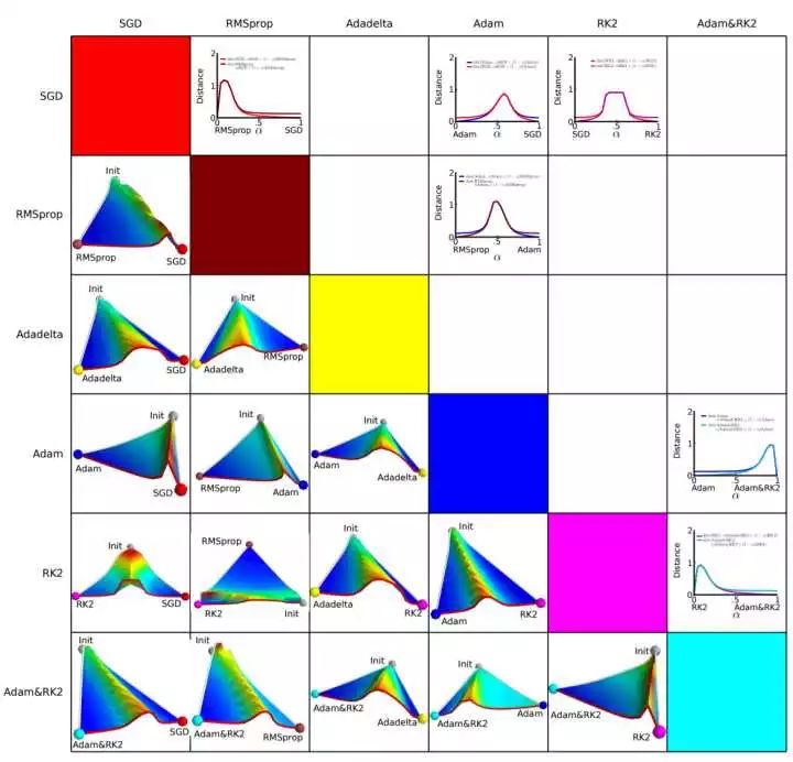
The above figure is the experimental result of the paper. The horizontal and vertical coordinates represent the feature space after dimensionality reduction, and the regional color indicates the change of the objective function value. Red is the plateau and blue is the depression. What they did was pairing experiments, letting the two algorithms start from the same initialization position and then comparing the results of the optimization. It can be seen that almost any two algorithms have come to different places, and they often have a very high plateau. This shows that different algorithms choose different descent directions when they are in the plateau.
▌08 Adam+SGD combination strategy
It is at every crossroads that the choice determines your destination. If God can give me a chance to come again, I will say to the girl: SGD!
The pros and cons of different optimization algorithms are still controversial topics that are not conclusive. According to the feedback I saw in paper and various communities, the mainstream view is that adaptive learning rate algorithms such as Adam have advantages for sparse data and fast convergence; but SGD (+Momentum) with fine tuning parameters can often be obtained. Better end result.
Then we will think, can we combine the two, first use Adam to quickly drop, then use SGD to tune, two birds with one stone? The idea is simple, but there are two technical problems:
When do you switch the optimization algorithm? - If the switch is too late, Adam may have already ran into his own basin, and SGD can't run any better.
What kind of learning rate is used after switching algorithms? - Adam uses the adaptive learning rate, which depends on the accumulation of second-order momentum. What kind of learning rate does SGD use for training?
The paper mentioned in the previous article, Improving Generalization Performance by Switching from Adam to SGD, proposes a solution to these two problems.
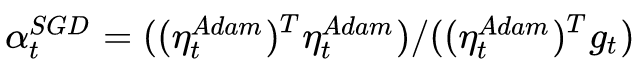
First look at the second question, the learning rate after switching.
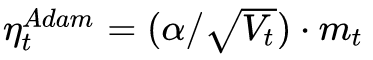
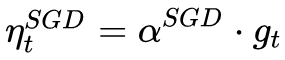
Adam’s down direction is
And the downward direction of SGD is
The SGD falling direction must be decomposed into the sum of the two directions of Adam's descent direction and its orthogonal direction, then its projection in the descending direction of Adam means the distance that SGD advances in the descending direction determined by the Adam algorithm. The projection in the orthogonal direction of the Adam's descending direction is the distance that the SGD advances in the correction direction of its choice.
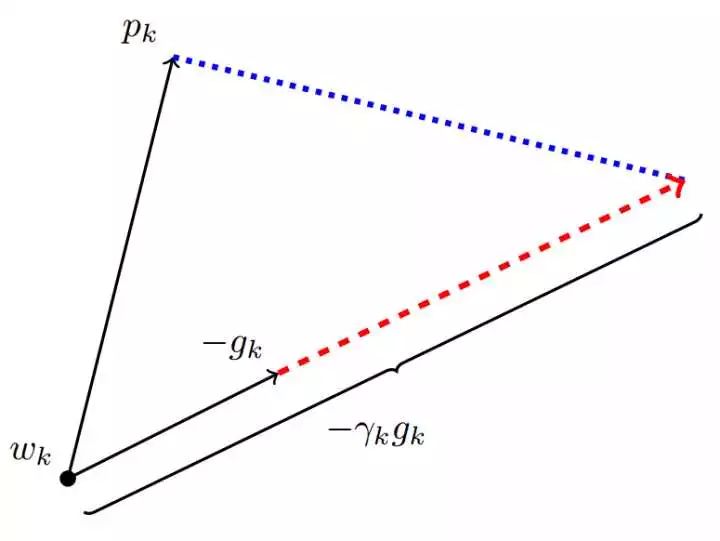
(The picture is from the original text, where p is the direction in which Adam descends, g is the direction of the gradient, and r is the learning rate of SGD.)
If SGD is going to finish the way that Adam has not finished, then first take over the banner of Adam - along  Take a step in the direction and then take the corresponding step along its orthogonal direction.
So we know how to determine the step size (learning rate) of the SGD - the orthogonal projection of the SGD in the direction of Adam's descent should be exactly equal to the direction of the drop in Adam (including the step size). That is:
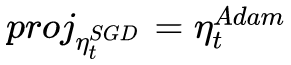
Solving this equation, we can get the learning rate of SGD:
To reduce the effects of noise, we can use the moving average to correct the estimate of the learning rate:
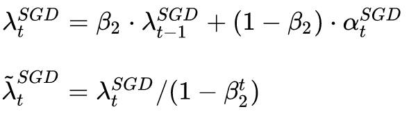
The beta parameter of Adam is directly reused here.
Then look at the first question, when to switch the algorithm.
The method proposed by the author is very simple, that is, when the moving average of the corresponding learning rate of SGD is basically unchanged, namely:
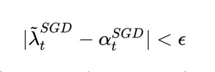
After each iteration, calculate the corresponding learning rate of the SGD successor. If it is found to be basically stable, then SGD will be  Going forward for the learning rate. However, this timing is not the optimal timing for switching. The author did not give a mathematical proof. It only verified the effect through experiments. The timing of switching is still a topic worthy of further study.
▌09 Common tricks for optimization algorithms
Finally, share some tricks in the selection and use of optimization algorithms.
1. First of all, the advantages and disadvantages of the major algorithms are inconclusive.
If you are just getting started, give priority to SGD+Nesterov Momentum or Adam. (Standford 231n : The two recommended updates to use are either SGD+Nesterov Momentum or Adam)
2. Choose the algorithm you are familiar with - so that you can use your experience more proficiently.
3. Fully understand your data - if the model is very sparse, then the algorithm of adaptive learning rate is prioritized.
4. Choose according to your needs. In the process of model design experiment, to quickly verify the effect of the new model, you can use Adam to perform rapid experiment optimization. Before the model is launched or the results are released, you can use the fine-tuned SGD to model. The ultimate optimization.
5. Experiment with small data sets first. Some papers have pointed out that the convergence speed of the stochastic gradient descent algorithm has little relationship with the size of the data set. (The mathematics of stochastic gradient descent are amazingly independent of the training set size. In particular, the asymptotic SGD convergence rates are independent from the sample size. [2]) Therefore, the experiment can be performed first with a representative small data set. Test the best optimization algorithms and find the optimal training parameters through parametric search.
6. Consider a combination of different algorithms. First use Adam to make a rapid drop, then switch to SGD for full tuning. The switching strategy can refer to the method described in this article.
7. The data set must be fully shuffled. In this way, when the adaptive learning rate algorithm is used, some feature sets can be avoided, and sometimes the problem of excessive deviation and sometimes insufficient learning leads to a deviation in the downward direction.
8. Continuously monitor the value of the objective function on the training data and verification data as well as the accuracy or changes in indicators such as AUC during the training. The monitoring of the training data is to ensure that the model is fully trained - the direction of decline is correct, and the learning rate is high enough; the monitoring data is monitored to avoid over-fitting.
9. Develop an appropriate learning rate decay strategy. Regular decay strategies can be used, such as attenuating each epoch; or using performance indicators such as accuracy or AUC to monitor the rate. When the indicator on the test set does not change or falls, the learning rate is reduced.
Here are just a few tricks on the optimization algorithm. If there are any omissions, you are welcome to add it to the comments. Thanks in advance!
A manual pulse generator (MPG) is a device normally associated with computer numerically controlled machinery or other devices involved in positioning. It usually consists of a rotating knob that generates electrical pulses that are sent to an equipment controller. The controller will then move the piece of equipment a predetermined distance for each pulse.
The CNC handheld controller MPG Pendant with x1, x10, x100 selectable. It is equipped with our popular machined MPG unit, 4,5,6 axis and scale selector, emergency stop and reset button.
Manual Pulse Generator,Handwheel MPG CNC,Electric Pulse Generator,Signal Pulse Generator
Jilin Lander Intelligent Technology Co., Ltd , https://www.landerintelligent.com